
Data wrangling, or data munging, involves transforming raw data into a desired format to enhance quality and usability for analytics or machine learning. A machine learning dataset serves as training data for algorithms to make predictions.

There are various methods to handle missing values in a machine-learning dataset. Mostly it depends on the type and amount of missing data and based on the analysis techniques carried out. Handling missing data is a crucial aspect of machine learning (ML) preprocessing, as it can significantly impact the performance and accuracy of models. Let us discuss some exciting methods to handle missing values in the ML dataset.
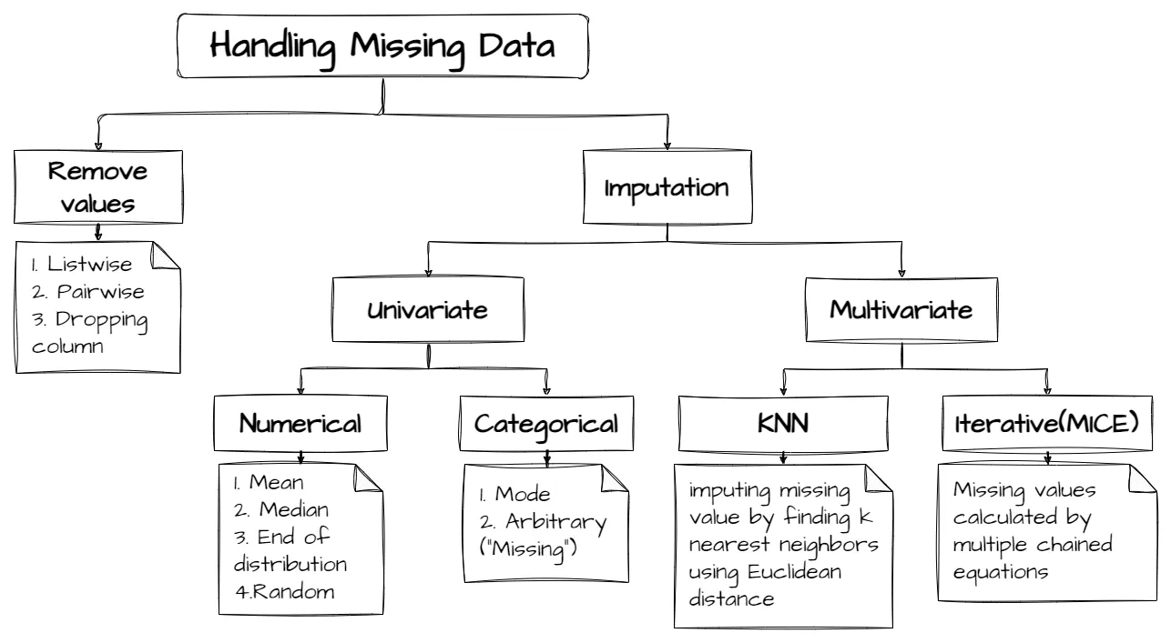
Removing values can sometimes be used in data analysis but cannot be used in machine learning since it may not give exact values. So, we have to deal with the missing data using other approaches.
1) Statistical Methods:
Mean imputation: Replace missing values with the mean of the variable.
Median imputation: Replace missing values with the median of the variable.

Mode imputation: Replace missing values with the most frequent value of the variable.
Mean Imputation:
- Replace missing values with the mean (average) of the variable.
Implementation:
- Calculate the mean of the variable and fill missing values with this mean.
Challenges:
- Can distort the distribution of the variable, mainly if there are extreme outliers.
- May not be suitable for variables with skewed distributions.
Key Features:
- Simple and easy to implement.
- Preserves the overall mean of the dataset.
Advantages:
- Preserves the overall trend of the data.
- Suitable for numerical variables with a normal distribution.
Disadvantages:
- May introduce bias, especially if missing values are not missing at random.
- Can underestimate variability if missingness is associated with extreme values.
Median Imputation:
- Replace missing values with the median (middle value) of the variable.
Implementation:
- Calculate the median of the variable and fill missing values with this median.
Challenges:
- Ignores extreme values, potentially affecting data distribution.
- May not be appropriate for variables with highly skewed distributions.
Key Features:
- Robust to outliers compared to mean imputation.
- Preserves the central tendency of the data.
Advantages:
- Less sensitive to extreme values compared to mean imputation.
- Suitable for variables with skewed distributions.
Disadvantages:
- Can still introduce bias if missingness is related to the median value.
- May not accurately represent the true variability of the data.
Mode Imputation:
- Replace missing values with the most frequent value of the variable.
Implementation:
- Calculate the mode (most frequent value) of the variable and fill missing values with this mode.
Challenges:
- Inadequate for continuous variables.
- Can lead to biased estimates if the mode is not representative of the variable’s distribution.
Key Features:
- Applicable for categorical variables.
- Preserves the mode of the variable.
Advantages:
- Simple and easy to implement for categorical data.
- Retains the most common value in the dataset.
Disadvantages:
- Unsuitable for continuous variables.
- May not be accurate if the mode does not represent the actual underlying distribution.
Mean, median, and mode imputation are commonly used methods for handling missing data in machine learning. Depending on the nature of the data and the requirements, it is essential to carefully consider each method’s implications and potential impact on the accuracy and reliability of the ML model.
2) K-Nearest Neighbors (KNN): Impute missing values based on the values of the K nearest neighbors.
Although KNN is primarily used for classification and regression tasks, it can also be adapted to handle missing data through imputation. The basic idea behind KNN imputation is to replace missing values in a dataset with the values of the K nearest neighbors.
Algorithm Overview:
- For each instance with missing values, the algorithm identifies its K nearest neighbors based on some distance metric.
- The missing values are then imputed using the values of the corresponding features from the nearest neighbors.
- The distance metric commonly used in KNN imputation is Euclidean distance, although other distance metrics like Manhattan distance or cosine similarity can also be employed.
Finding Nearest Neighbors:
- Nearest neighbors are determined based on the similarity of feature values.
- The distance between instances is calculated using the chosen distance metric.
- The K nearest neighbors are the instances with the smallest distances to the example with missing values.
Imputation Process:
- Once the K nearest neighbors are identified, the missing values are imputed by taking the average (for numeric features) or the mode (for categorical features) of the corresponding feature values from these neighbors.
- If there is a tie in the mode for categorical features, a random value may be selected among the modes.
Key Features of KNN Imputation:
Non-parametric Approach:
- KNN imputation does not make assumptions about the underlying data distribution, making it suitable for various types of datasets.
Adaptability:
- KNN can handle both numeric and categorical features, making it versatile for different types of data.
Local Information Utilization:
- It imputes missing values based on local neighborhood information rather than the entire dataset, which can capture local patterns effectively.
Challenges of KNN Imputation:
Computational Complexity:
- As the dataset size increases, the computational cost of finding nearest neighbors grows, impacting performance.
Determining K:
- Selecting the appropriate value of K can be challenging and may affect imputation accuracy. A small K may lead to overfitting, while a large K may introduce bias.
Advantages of KNN Imputation:
Preservation of Local Patterns:
- KNN imputation preserves local data patterns, which may be beneficial for maintaining data integrity.
Robustness:
- It is robust to outliers and noisy data, as it relies on a voting mechanism among neighbors.
Disadvantages of KNN Imputation:
Sensitivity to Distance Metric:
- The choice of distance metric can significantly impact imputation results, requiring careful selection.
Data Sparsity:
- In high-dimensional spaces or with sparse data, finding meaningful neighbors can be challenging, leading to less accurate imputations.
KNN imputation is a flexible method for handling missing data in machine learning, leveraging local neighborhood information to impute missing values.
3) Regression imputation
This method is used to handle missing data in machine learning by replacing missing values with predicted values based on a regression model.
Algorithm Overview:
- Regression imputation involves fitting a regression model to the dataset, where the target variable is the feature with the missing values, and the predictor variables are the other features in the dataset.
- Once the regression model is trained, it can be used to predict missing values for the target feature based on the observed values of the predictor features.
Regression Model Selection:
- The choice of regression model depends on the nature of the data and the relationship between variables.
- Standard regression models used for imputation include linear regression, polynomial regression, decision tree-based models (e.g., random forests), and more complex models like support vector regression or neural networks.
Imputation Process:
- Once the regression model is trained, missing values for the target feature are replaced with the predicted values obtained from the regression model.
- The predicted values are calculated based on the values of the predictor features for each instance with missing data.
Key Features of Regression Imputation:
Flexibility: Regression imputation can handle both numeric and categorical target variables, making it versatile for different types of data.
Use of Relationships: It leverages the relationships between variables in the dataset to impute missing values, capturing more complex patterns compared to more straightforward imputation methods.
Prediction Accuracy: The accuracy of imputed values depends on the performance of the regression model, allowing for potentially more accurate imputations with well-performing models.
Challenges of Regression Imputation:
Model Selection: Selecting an appropriate regression model can be challenging and may require experimentation to find the best-performing model for the dataset.
Overfitting: There is a risk of overfitting if the regression model captures noise or irrelevant patterns in the data, leading to poor generalization performance.
Bias: The imputed values may introduce bias if the regression model fails to capture the underlying relationships between variables accurately.
Advantages of Regression Imputation:
Preservation of Relationships: Regression imputation preserves the relationships between variables in the dataset, leading to more realistic imputed values.
Handling Multivariate Imputation: It can handle imputation of missing values for multiple variables simultaneously by considering all predictor features in the regression model.
Disadvantages of Regression Imputation:
Complexity: Training a regression model can be computationally expensive, particularly for large datasets or complex models.
Assumption of Linearity: Linear regression-based imputation assumes a linear relationship between variables, which may not always hold true for the data.
Sensitivity to Outliers: Outliers in the dataset can disproportionately influence the regression model’s predictions, leading to potentially biased imputations.
Regression imputation is a flexible method for handling missing data in machine learning, leveraging regression models to predict missing values based on the relationships between variables.
4) Interpolation method
Interpolation is a method used to estimate missing values in a dataset by extrapolating existing data points. In the context of handling missing data in machine learning (ML), interpolation techniques are applied when some values are absent, but there is a clear trend or pattern in the available data. Interpolation aims to fill in the missing values based on the relationship between neighboring data points.
Types of Interpolation:
Linear Interpolation: Assumes a linear relationship between neighboring data points and estimates missing values accordingly.
Polynomial Interpolation: Fits a polynomial curve to the data and uses it to predict missing values.
Spline Interpolation: Utilizes piecewise polynomial functions to interpolate between data points, providing a smoother curve.
Interpolation Process:
- Identify missing values in the dataset.
- Determine neighboring data points surrounding the missing values.
- Apply the chosen interpolation method to estimate the missing values based on the known data points.
Key Features of Interpolation Method:
Preservation of Data Trends: Interpolation preserves the underlying trends and patterns present in the dataset, ensuring that the estimated values align with the overall data distribution.
Flexible Application: Interpolation techniques can be applied to both numerical and categorical data, making them versatile for various types of datasets.
Simplicity: Interpolation methods are relatively straightforward to implement and understand, requiring minimal computational resources.
Challenges of Interpolation Method:
Sensitivity to Outliers: Interpolation techniques may produce inaccurate estimates if outliers are present in the dataset, as they can distort the underlying trends.
Assumption of Linearity: Linear interpolation assumes a linear relationship between data points, which may not always hold true for complex datasets with nonlinear patterns.
Overfitting: Polynomial interpolation, in particular, may lead to overfitting if the degree of the polynomial is too high, resulting in poor generalization performance.
Advantages of Interpolation Method:
Efficiency: Interpolation can quickly estimate missing values without requiring extensive computational resources or complex algorithms.
Preservation of Data Structure: Interpolation methods ensure that the imputed values maintain the structure and integrity of the original dataset, minimizing potential distortions.
Versatility: Interpolation techniques can be easily customized and adapted to suit different types of datasets and analytical requirements.
Disadvantages of Interpolation Method:
Limited Accuracy: Interpolation methods may yield less accurate estimates for missing values compared to more sophisticated imputation techniques, especially in datasets with irregular patterns or significant outliers.
Risk of Bias: Interpolation may introduce bias if the missing values are not missing completely at random (MCAR) or if there are systematic errors in the data.
Complexity Consideration: While linear interpolation is simple, more advanced interpolation methods like polynomial or spline interpolation require careful consideration of parameters and may be prone to overfitting.
Interpolation is a valuable method for handling missing data in ML, mainly when there is a clear trend or pattern in the available data. While it offers advantages such as simplicity and preservation of data structure, challenges such as sensitivity to outliers and limited accuracy need to be carefully addressed for optimal performance.
5) Exploratory Data Analysis (EDA)
Exploratory Data Analysis (EDA) is a crucial method in data science and machine learning for understanding the structure, patterns, and relationships within a dataset. While EDA itself doesn’t handle missing data directly, it’s an essential preliminary step that involves identifying, visualizing, and analyzing missing values to inform subsequent data handling strategies.
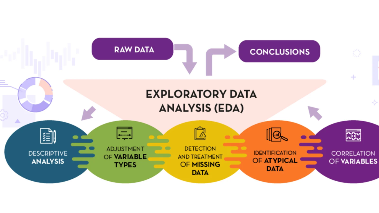
Key Features of EDA:
Visualization: EDA utilizes various graphical techniques such as histograms, scatter plots, and heatmaps to visualize missing data patterns, enabling easy identification of missing values and their distribution across variables.
Statistical Summaries: EDA provides descriptive statistics like counts, percentages, and correlations to quantify the extent and impact of missing values in the dataset, facilitating informed decision-making on how to handle them.
Pattern Recognition: EDA helps identify potential patterns or relationships between missing values and other variables, which can inform imputation strategies or shed light on underlying data collection issues.
Data Cleaning Guidance: EDA informs the selection of appropriate missing data handling techniques based on the nature and distribution of missing values, ensuring the integrity and reliability of the subsequent analysis.
Challenges of EDA:
Complexity of Data: EDA can be challenging for large, high-dimensional datasets with complex structures, as it may require specialized techniques and tools to visualize and analyze missing data patterns effectively.
Biased Interpretations: Without careful consideration, EDA results may lead to biased interpretations or incorrect conclusions if missing data patterns are not properly understood or accounted for.
Time and Resource Intensive: Conducting comprehensive EDA can be time-consuming and resource-intensive, particularly for datasets with extensive missing values or diverse variable types.
Advantages of EDA:
Data Understanding: EDA provides valuable insights into the characteristics and quality of the dataset, helping researchers and analysts understand its strengths, limitations, and potential biases.
Early Detection of Issues: EDA enables early detection of missing data issues, allowing researchers to address them proactively and improve the overall quality and reliability of the analysis.
Informed Decision-Making: EDA guides decision-making on how to handle missing data by providing evidence-based insights into the distribution, patterns, and potential impact of missing values on the analysis.
Disadvantages of EDA:
Subjectivity: EDA interpretation can be subjective, as it relies on the analyst’s judgment and expertise to identify relevant patterns and relationships in the data, which may introduce bias or inconsistency.
Limited Scope: EDA is primarily descriptive and exploratory, focusing on uncovering patterns and trends within the existing data, rather than generating new hypotheses or causal relationships.
Potential Overlook of Complex Relationships: In complex datasets, EDA may oversimplify or overlook intricate relationships between variables, leading to incomplete or misleading conclusions about missing data patterns.
Exploratory Data Analysis is a critical method for understanding missing data in machine learning. While it offers valuable insights and guidance for handling missing values, challenges such as data complexity and interpretation subjectivity need to be carefully addressed to ensure robust and reliable analysis outcomes.
6) Data cleaning with Pandas
Data cleaning with Pandas is a fundamental technique in handling missing data within Python’s Pandas library, commonly used in machine learning (ML) workflows. Pandas offers a comprehensive set of functions and methods for efficiently managing missing values in datasets. Here’s a detailed explanation of data cleaning with Pandas, including its key features, challenges, advantages, and disadvantages:
Key Features of Data Cleaning with Pandas:
Missing Value Identification: Pandas provides functions like .isnull() and .notnull() to detect missing values in datasets, allowing users to locate and quantify the extent of missingness.
Missing Value Handling:
Imputation: Replacing missing values with a specified value (e.g., mean, median, mode).
Deletion: Removing rows or columns with missing values using .dropna() method.
Interpolation: Filling missing values using methods like .interpolate().
Customized Handling: Users can define custom functions for handling missing values based on specific data characteristics.
Data Integration: Pandas seamlessly integrates with other Python libraries and tools commonly used in ML workflows, such as NumPy, Scikit-learn, and Matplotlib, enabling efficient data preprocessing and analysis.
Efficient Data Manipulation: Pandas provides powerful data manipulation capabilities, including indexing, slicing, grouping, and aggregation, facilitating complex data cleaning operations on large datasets.
Challenges of Data Cleaning with Pandas:
Data Quality Assurance: While Pandas offers various tools for handling missing values, ensuring the accuracy and reliability of imputed values can be challenging, especially in the absence of domain knowledge.
Computational Complexity: Performing data cleaning operations on large datasets can be computationally intensive and time-consuming, requiring efficient algorithms and optimization techniques to maintain performance.
Subjectivity in Imputation: Choosing appropriate imputation methods involves subjective judgment and may introduce bias, especially if the chosen method does not accurately represent the underlying data distribution.
Advantages of Data Cleaning with Pandas:
Ease of Use: Pandas provides an intuitive and user-friendly interface for handling missing data, making it accessible to both novice and experienced users.
Flexibility: Pandas offers a wide range of functions and methods for handling missing values, allowing users to customize data cleaning strategies based on specific requirements and preferences.
Integration with ML Pipelines: Data cleaned using Pandas can be seamlessly integrated into ML pipelines for model training, evaluation, and deployment, streamlining the end-to-end ML workflow.
Disadvantages of Data Cleaning with Pandas:
Limited Scalability: While Pandas is efficient for working with moderately sized datasets, it may struggle with larger datasets due to memory constraints and computational overhead.
Potential Overfitting: Imputation methods employed in Pandas may lead to overfitting if not carefully validated, potentially compromising the generalization performance of ML models.
Complexity in Handling Multivariate Missingness: Pandas may not offer built-in solutions for handling complex missing data patterns involving multiple variables, requiring users to implement custom solutions.
Data cleaning with Pandas is a versatile and efficient method for handling missing data in ML workflows. While it offers numerous advantages, challenges such as data quality assurance and computational complexity need to be carefully addressed to ensure accurate and reliable data preprocessing.
7) Algorithm usage to assist missing data
Using algorithms to assist in handling missing data is a common approach in machine learning (ML), where sophisticated models are employed to predict missing values based on the available data. This method leverages the relationship between the observed features and the target feature with missing values to estimate or impute the missing data.
Key Features of Algorithm Usage for Missing Data:
Predictive Modeling: Algorithms such as regression, decision trees, random forests, and neural networks are used to build predictive models that estimate missing values based on other features in the dataset.
Model Training: The dataset with complete cases is used to train the predictive model, where the target variable is the feature with missing values, and the predictor variables are the features with complete data.
Prediction: Once the model is trained, it is used to predict missing values in the dataset based on the observed values of other features, effectively imputing the missing data points.
Evaluation: The performance of the predictive model is evaluated using metrics such as mean absolute error, mean squared error, or accuracy, to ensure the reliability and accuracy of the imputed values.
Challenges of Algorithm Usage for Missing Data:
Model Selection: Choosing the appropriate algorithm for imputation depends on the dataset characteristics, including the nature of missingness, the distribution of data, and the relationships between variables.
Overfitting: Predictive models may overfit the training data, capturing noise or irrelevant patterns, which can lead to inaccurate imputations and poor generalization performance on unseen data.
Complexity: Some algorithms may be computationally expensive and resource-intensive, particularly for large datasets or models with a high number of features.
Advantages of Algorithm Usage for Missing Data:
Data-driven Imputation: Algorithms leverage the data’s inherent structure and patterns to estimate missing values, resulting in more accurate imputations compared to simple methods like mean imputation.
Adaptability: Algorithms can handle various types of missing data patterns, including missing completely at random (MCAR), missing at random (MAR), and missing not at random (MNAR), making them versatile for different datasets.
Integration with ML Pipelines: Imputation algorithms seamlessly integrate with ML pipelines, allowing imputed datasets to be directly used for model training, evaluation, and prediction.
Disadvantages of Algorithm Usage for Missing Data:
Complexity and Resource Intensiveness: Building and training predictive models for imputation can be complex and resource-intensive, requiring expertise in machine learning and computational resources.
Model Assumptions: Imputation algorithms may make assumptions about the underlying data distribution or relationships between variables, which may not always hold true in practice, leading to biased imputations.
Risk of Error Propagation: Inaccurate imputations can propagate errors and bias into downstream analyses or model predictions, potentially compromising the validity and reliability of the results.
Using algorithms to assist with missing data in ML offers several advantages, including data-driven imputation and adaptability to different datasets. However, challenges such as model selection, overfitting, and computational complexity need to be carefully addressed to ensure accurate and reliable imputations.
After carefully analysing the types of methods used to handle missing data in Machine Learning Dataset, a single or multiple methods can be chosen based on the user requirements.